Singular Value Decompositions (SVD) have become very popular in the field of Collaborative Filtering. The winning entry for the famed Netflix Prize had a number of SVD models including SVD++ blended with Restricted Boltzmann Machines.
However, I’ve been confused by the implementation of SVD for a long time and decided to gain a deeper understanding of it. Here are my notes on SVD.
I think one of the most impressive thing in linear algebra is the connection between purely matrix and linear transformation in a complex space.
The singular value decomposition
Let’s say if we have a 2 * 2 matrix.
The geometric essence of the singular value decomposition for 2 * 2 matrices: for any 2 * 2 matrix, we may find an orthogonal grid that is transformed into another orthogonal grid.
We will express this fact using vectors: with an appropriate choice of orthogonal unit vectors v1 and v2, the vectors Mv1 and Mv2 are orthogonal.
We will use u1 and u2 to denote unit vectors in the direction of Mv1 and Mv2. The lengths of Mv1 and Mv2 - - denoted by σ1 and σ2 - - describe the amount that the grid is stretched in those particular directions. These numbers are called the singular values of M.
Therefore,
\(M v_1 = \sigma_1 u_1\)
\(M v_2 = \sigma_2 u_2\)
We may now give a simple description for how the matrix M treats a general vector x. Since the vectors v1 and v2 are orthogonal unit vectors, so
\(Mx = (v_1x)Mv_1 + (v_2x)Mv_2 \)
\(Mx = (v_1x)\sigma_1 u_1 + (v_2x) \sigma_2 u_2 \)
which leads to
\(Mx = u_1 \sigma_1 v_1^Tx + u_2 \sigma_2 v_2^Tx \)
\(M = u_1 \sigma_1 v_1^T + u_2 \sigma_2 v_2^T \)
usually expressed by
\(M = U \Sigma V^T\)
Applications
Data compression
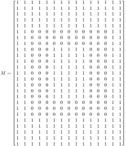
Singular value decompositions can be used to represent data efficiently. Suppose, for instance, that we wish to transmit the following image, which consists of an array of 15 * 25 black or white pixels.

We will represent the image as a 15 * 25 matrix in which each entry is either a 0, representing a black pixel, or 1, representing white. As such, there are 375 entries in the matrix.

if we perform a singular value decomposition on M, we find there are only three non-zero singular values.
σ1 = 14.72
σ2 = 5.22
σ3 = 3.31
Therefore, the matrix may be represented as
\(M = u_1 \sigma_1 v_1^T + u_2 \sigma_2 v_2^T + u_3 \sigma_3 v_3^t \)
This means that we have three vectors vi, each of which has 15 entries, three vectors ui, each of which has 25 entries, and three singular values σi. This implies that we may represent the matrix using only 123 numbers rather than the 375 that appear in the matrix. In this way, the singular value decomposition discovers the redundancy in the matrix and provides a format for eliminating it.
Noise reduction
Typically speaking, the large singular values point to where the interesting information is. For example, imagine we have used a scanner to enter this image into our computer. However, our scanner introduces some imperfections in the image.

We may proceed in the same way: represent the data using a 15 * 25 matrix and perform a singular value decomposition. We find the following singular values:
σ1 = 14.15
σ2 = 4.67
σ3 = 3.00
σ4 = 0.21
σ5 = 0.19
…
σ15 = 0.05
Clearly, the first three singular values are the most important so we will assume that the others are due to the noise in the image and make the approximation
\(M \approx u_1 \sigma_1 v_1^T + u_2 \sigma_2 v_2^T + u_3 \sigma_3 v_3^t \)
This leads to an improved image.
References:
Dan Kalman, A Singularly Valuable Decomposition: The SVD of a Matrix, The College Mathematics Journal 27 (1996), 2-23.
comments powered by Disqus