Recently, as planning to do some project related to deep learning (specifically image classification, detection etc.) in the near future, I spent some time dig into this field.
Based on the previous understanding of linear algebra, calculus, statistics and a few knowledge about machine learning, I had a tiny bit of conceptual understanding of deep learning, though I was completely unable to transfer any of my knowledge into code.
This is what I wanted to change.
Why Keras?
The framework I started with is Keras. Keras is an actual deep learning framework: a well-designed API that allows you use to build deep learning models by clipping together high-level building blocks. And since Keras runs on top of TensorFlow or Theano , there is no performance cost to using Keras compared to using the one of these lower-level frameworks.
If you are familiar with Numpy and Scikit-Learn, then a fair comparison would be to say that Theano and TensorFlow are closer to Numpy, while Keras is closer to Scikit-Learn.
However the comparison isn’t perfect, since Keras is more flexible than Scikit-Learn: it allows you to define your own machine learning models, rather than just use pre-defined models. As for Torch, Keras has a significantly larger community than Torch, we can benefit from the extensive Python ecosystem in our workflow.
Build a neural network with Keras
Load dataset.
import numpy as np
import matplotlib.pyplot as plt
from keras.datasets import mnist
from keras.models import Sequential
from keras.layers.core import Dense, Dropout, Activation
from keras.utils import np_utils
Using TensorFlow backend.
nb_classes = 10

# the data, shuffled and split between tran and test sets
(X_train, y_train), (X_test, y_test) = mnist.load_data() #
print("X_train original shape", X_train.shape)
print("y_train original shape", y_train.shape)
X_train original shape (60000, 28, 28)
y_train original shape (60000,)
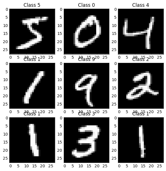
Take a look at some examples of the training data.
for i in range(9):
    plt.subplot(3,3,i+1)
    plt.imshow(X_train[i], cmap='gray', interpolation='none')
    plt.title("Class {}".format(y_train[i]))
plt.show()
Format the data for training.
X_train = X_train.reshape(60000, 784)
X_test = X_test.reshape(10000, 784)
X_train = X_train.astype('float32')
X_test = X_test.astype('float32')
X_train /= 255
X_test /= 255
print("Training matrix shape", X_train.shape)
print("Testing matrix shape", X_test.shape)
Training matrix shape (60000, 784)
Testing matrix shape (10000, 784)
Y_train = np_utils.to_categorical(y_train, nb_classes)
Y_test = np_utils.to_categorical(y_test, nb_classes)
Build the neural-network. Here we’ll do a simple 3 layer fully connected network.
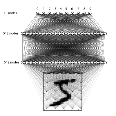
model = Sequential()
model.add(Dense(512, input_shape=(784,)))
model.add(Activation('relu'))

model.add(Dropout(0.2))   # Dropout helps protect the model from memorizing or "overfitting" the training data

model.add(Dense(512))
model.add(Activation('relu'))

model.add(Dropout(0.2))

model.add(Dense(10))
model.add(Activation('softmax'))
When compiing a model, Keras asks you to specify your loss function and your optimizer. The loss function we’ll use here is called categorical crossentropy, and is a loss function well-suited to comparing two probability distributions.
model.compile(loss='categorical_crossentropy',metrics=["accuracy"], optimizer='adam')
Train the model.
model.fit(X_train, Y_train,
          batch_size=128, nb_epoch=4,
          verbose=1,
          validation_data=(X_test, Y_test))
Train on 60000 samples, validate on 10000 samples
Epoch 1/4
60000/60000 [==============================] - 15s - loss: 0.2492 - acc: 0.9254 - val_loss: 0.1199 - val_acc: 0.9615
Epoch 2/4
60000/60000 [==============================] - 15s - loss: 0.0991 - acc: 0.9691 - val_loss: 0.0807 - val_acc: 0.9736
Epoch 3/4
60000/60000 [==============================] - 15s - loss: 0.0711 - acc: 0.9773 - val_loss: 0.0922 - val_acc: 0.9712
Epoch 4/4
60000/60000 [==============================] - 15s - loss: 0.0541 - acc: 0.9826 - val_loss: 0.0670 - val_acc: 0.9787

<keras.callbacks.History at 0x119233b70>
Finally, evaluate its performance
score = model.evaluate(X_test, Y_test,verbose=0)
print('Test score:', score[0])
print('Test accuracy:', score[1])
Test score: 0.0669518932859
Test accuracy: 0.9787
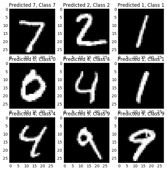
Inspecting the output
predicted_classes = model.predict_classes(X_test)

# Check which items we got right / wrong
correct_indices = np.nonzero(predicted_classes == y_test)[0]
incorrect_indices = np.nonzero(predicted_classes != y_test)[0]
9952/10000 [============================>.] - ETA: 0s
plt.figure()
for i, correct in enumerate(correct_indices[:9]):
plt.subplot(3,3,i+1)
plt.imshow(X_test[correct].reshape(28,28), cmap='gray', interpolation='none')
plt.title("Predicted {}, Class {}".format(predicted_classes[correct], y_test[correct]))
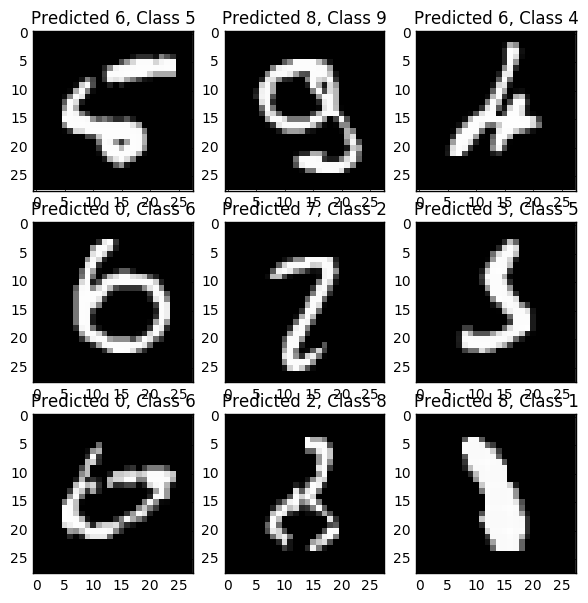
plt.figure()
for i, incorrect in enumerate(incorrect_indices[:9]):
plt.subplot(3,3,i+1)
plt.imshow(X_test[incorrect].reshape(28,28), cmap='gray', interpolation='none')
plt.title("Predicted {}, Class {}".format(predicted_classes[incorrect], y_test[incorrect]))
plt.show()